
In this section we will explore and visualize Echo Nest genres using graphs.
The graph will be constructed using all the 1373 genres and their relations provided
from the Echo Nest API. The Python networkx module is used to create
the directed graph. Here each node will represent a genre and each edge between
nodes will be made based on Echo Nest similarity finder. The similarity finder
provided form Echo Nest, finds similar genres to a given genre, e.g. the genre
Metal is similar to Speed Metal, Thrash Metal, Death Metal, Power Metal,
Nwobhm, Progressive Metal, Hard Rock, Melodic Death Metal, Neo Classical
Metal, Rock, Crossover Thrash, Melodic Metalcore, Viking Metal, Black Metal
and Groove Metal. For each similar genre a similarity measure is provided showing
how much the two genres are similar. This is used as weights on the edges.
A directed graph is used since it is possible for a similarity to go from one genre
to another and not back again.
The purpose of the graph is to visualize the relationships between the different
genres given from Echo Nest.
The created graph contains 1373 nodes and 5718 edges. From this 115 nodes
are found to have no degree, these are remove since they do not provide any information regrading the genres connections. This gives us a final graph of 1258 nodes
and 5718 edges. The graph is imported to Gephi
, where we rank,
partition and create a layout of the graph. We rank each node by it’s total in and out
degree, so genres that have many similar genres and other genres are similar to,
is shown bigger. By running the build-in statistics in Gephi we find the average
degree to be 4.55. The graphs colouring is based on it’s Modularity class,
thereby getting classes where there is a strong cluster of connections between
genres. From this we found 96 different modularity classes in total, each
represented with its own color. The biggest cluster contains 8.66% of the nodes
in the total graph. The layout of the graph is based on the Fruchterman Reingold algorithm because we estimate this gives the best overview of the graph.
In addition to this we are also removing all notes that are not connected
with the biggest component in the graph. We do this since we found that
small clusters that were disconnected from the biggest component were strongly
connected through culture or/and language basis, as the cluster shown below.
 This then gives us a connected graph with 965 nodes and 5156 edges, and 20
different Modularity classes, with the biggest cluster representing 11.81% of the
final graph. The graph can be found below.
This then gives us a connected graph with 965 nodes and 5156 edges, and 20
different Modularity classes, with the biggest cluster representing 11.81% of the
final graph. The graph can be found below.

The graph below is provides the most information if it is explored in depth.
The controls for doing so are best learned by trial and error. For others who like to do things by the book, the controls are as follows:
- Move: Press and hold
- Zoom: Mouse wheel or double click
- Will reveal smaller labels
- View node label: Hover node
- Highlight neigbors: Click node
We now export the graph back to Python to make some analysis on the graph. From the graph we find the genres with the 10 biggest in and out going degree. The results is shown in the table below.
| Genre & In degree | Genre & Out degree |
|---|---|
| Alternative Rock, 36 | Folk rock, 15 |
| Indie Rock, 33 | Classic rock, 15 |
| Soul Blues, 31 | Alternative Rock, 15 |
| Folk Christmas, 30 | Glam Rock, 15 |
| Rock, 30 | Funk, 15 |
| Jazz Christmas, 26 | Jazz Christmas, 15 |
| Lo-fi, 26 | Pagan Black Metal, 15 |
| Folk-Pop, 26 | Jazz Blues, 15 |
| Singer-Songwriter, 25 | Neo-Psychedelic, 15 |
| Jazz Blues, 23 | Noise Pop, 15 |
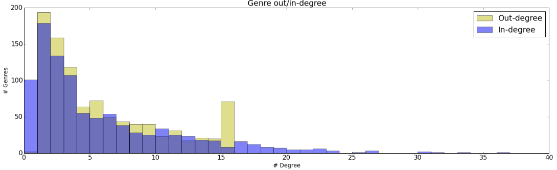 From the Figure we see that the in degree is exponential decreasing after 1,
we also see that there is almost no genres with 0 out degree, this means that
almost all genres are similar to minimum one other genre. We also see that a
genre max can have 15 out going degrees. besides this we see the distribution of
numbers of genres with in and out degree is almost the same, with out degree
being a little bit higher.
We now run the Betweenness Centrality on the graph to see which genres
that are important. Betweenness Centrality is equal to the number of shortest
paths form all genres to all other paths that passes through that genre. The
10 first most important genres from the Betweenness Centrality is shown in the
table below.
From the Figure we see that the in degree is exponential decreasing after 1,
we also see that there is almost no genres with 0 out degree, this means that
almost all genres are similar to minimum one other genre. We also see that a
genre max can have 15 out going degrees. besides this we see the distribution of
numbers of genres with in and out degree is almost the same, with out degree
being a little bit higher.
We now run the Betweenness Centrality on the graph to see which genres
that are important. Betweenness Centrality is equal to the number of shortest
paths form all genres to all other paths that passes through that genre. The
10 first most important genres from the Betweenness Centrality is shown in the
table below.
| Genre | Betweenness Centrality score |
|---|---|
| Punk | 0.1243 |
| Ska Punk | 0.1203 |
| Ska Revival | 0.1164 |
| Rock Steady | 0.1150 |
| World Christmas | 0.0991 |
| Latin Christmas | 0.0950 |
| Experimental | 0.0707 |
| Drone | 0.0697 |
| Protopunk | 0.0688 |
| Minimal | 0.0588 |
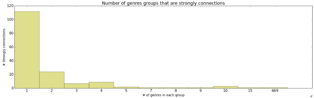 From the Figure we see that we have one group contains 669 of all the genres,
and we have 112 groups containing only one genre.
From the Figure we see that we have one group contains 669 of all the genres,
and we have 112 groups containing only one genre.